Products & Technology
Featured Ecosystems
Company
Breaking Down Proof Construction in Plonky3: The Fibonacci Example Unveiled
ZKVM and Plonky3
In recent years, zero-knowledge Virtual Machines (zkVMs) have emerged as a transformative innovation in blockchain technology. They enable anyone to prove that a program was executed correctly on specific inputs, without revealing the inputs themselves, offering a powerful framework for secure and private computation at scale.
A critical component driving zkVMs is the underlying proof system. Among the most prominent is Polygon’s Plonky3, a state-of-the-art prover that powers several leading zkVM projects. Plonky3 is particularly valued for its efficiency in generating proofs quickly, a property essential for making zkVMs practical in real-world applications.
Despite its importance, Plonky3 is often treated within zkVM architectures as a black-box proof engine. Most tutorials and developer guides emphasize writing constraints, while abstracting away the internals of the proving process. While this abstraction lowers the barrier to entry, it can obscure the deeper mechanics and limit opportunities for optimization or customization in specialized domains.
In this post, we will take a closer look inside Plonky3’s proving phase, using the classical example of a Fibonacci circuit. We assume readers have a basic understanding of STARKs (Scalable Transparent ARguments of Knowledge) and aim to provide a clear walkthrough of how Plonky3 constructs and generates proofs, shedding light on the process behind the prover that powers many zkVMs.
Workflow of Plonky3: A Gentle Technical Introduction
Plonky3 is a proving toolkit that provides core primitives, such as Polynomial Commitment Schemes (PCS), to implement Polynomial IOPs (PIOPs). At its core, Plonky3 leverages a highly optimized STARK prover, along with its variant, Circle STARK.
For readers new to this field, we recommend starting with STARK 101 by StarkWare. For those who want to dive deeper, resources such as Lambdaclass’s documentation or the ethSTARK paper provide excellent technical details and even reference implementations.
At a high level, a STARK (and its Plonky3 implementation) consists of two foundational layers:
- Arithmetization system
- Proving system
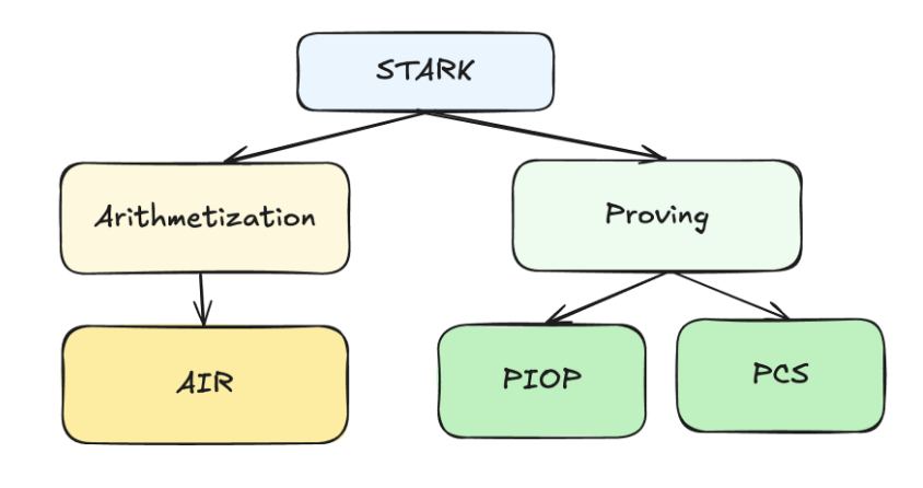
Arithmetization: Algebraic Intermediate Representation (AIR)
In STARKs, the arithmetization layer is expressed through the Algebraic Intermediate Representation (AIR). AIR encodes a computation (e.g., program execution) into a set of algebraic constraints, usually represented as polynomial equations.
Concretely, the AIR describes a computation trace: a sequence of steps where each step is linked by transition rules. You can picture this trace as a matrix(or a table), where each column represents a state register (much like in a CPU); we will explore this structure in detail later in our example. These rules enforce consistency in the trace by specifying polynomial relationships between the values at different steps of execution.
Proving Layer: PIOP + PCS
The proving system in STARKs (and Plonky3) builds on two key primitives:
- Polynomial IOP (Interactive Oracle Proof): This defines the rules of the "Q&A game." In this theoretical model, the Prover doesn't send the entire polynomial. Instead, they grant the Verifier access to a magical "oracle"—a black box that can instantly answer queries like, "What is the polynomial's value at a specific point?" The Verifier interacts with this conceptual oracle to verify the Prover's honesty without learning the entire polynomial, thereby ensuring the correctness of the trace.
- Polynomial Commitment Scheme (PCS): A PCS is the real-world cryptographic tool that instantiates the oracle described in the PIOP model. Since magical black boxes don't exist, we need a concrete way to create a binding, verifiable promise. The PCS does exactly that: - The Prover uses the PCS to "commit" to the polynomial, creating a short digital fingerprint (like a Merkle root). This fingerprint acts as the public, trustworthy handle for the oracle. - Later, the Prover can "open" the commitment at any point the Verifier chooses, providing a value and a proof that this value is consistent with the original fingerprint. This is the secure mechanism for "answering the oracle's query."
Together, these components enable succinct, verifiable proofs of large computations.
Workflow of Plonky3’s STARK
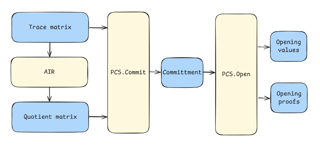
The proof construction process in Plonky3 generally follows this workflow:
- Generate Trace: The prover executes the computation and records the corresponding execution trace matrix. This trace is the raw evidence of the entire computation, from start to finish.
- Commit Trace: The prover commits to the execution trace using a PCS, i.e., a Merkle root of the trace matrix.
- Compute & Commit Quotients: The prover must prove that the evidence follows all the rules (the constraints). Using the "division trick" we will discuss later, prover creates a new, special polynomial called the quotient polynomial, then commits it.
- Open Polynomials: Using the PCS, the prover opens both the trace polynomials and combined quotient polynomials at verifier-chosen points.
- Verify Proofs: The verifier checks the commitments and openings(both opening values and opening proofs) to validate the correctness of the proof. If it does, they are convinced that the Prover's entire, massive computation was performed correctly.
A Guided Example: Fibonacci Sequence
In the next section, we will walk through a simple yet illustrative example: proving the correctness of Fibonacci computations. The Fibonacci sequence is familiar and mathematically straightforward, making it a perfect entry point to understand how Plonky3 constructs proofs.
We will also introduce supporting formulas and diagrams to illustrate the workflow. While these visual aids may abstract away some of the finer technical details, they are designed to highlight the essential mechanics of how Plonky3’s proof system operates in practice.
Use Plonky3 to Prove Fibonacci
We adapted the Plonky3 Fibonacci example to work with the latest version of Plonky3. For simplicity, we use the 2-adic PCS instead of Circle PCS. While Circle PCS offers additional optimizations, the 2-adic version is easier for newcomers to follow, especially if you already have some background in STARKs.
If you’re looking for detailed explanations of configuration parameters and core components, the README.md of the repository is an excellent resource. It covers the foundational concepts and setup in depth, making it useful for both beginners and readers seeking a deeper dive.
The following is the execution log from our example. After most function calls, you’ll notice that the matrix dimensions (i.e., evaluations of polynomials) are displayed, for example, dims:
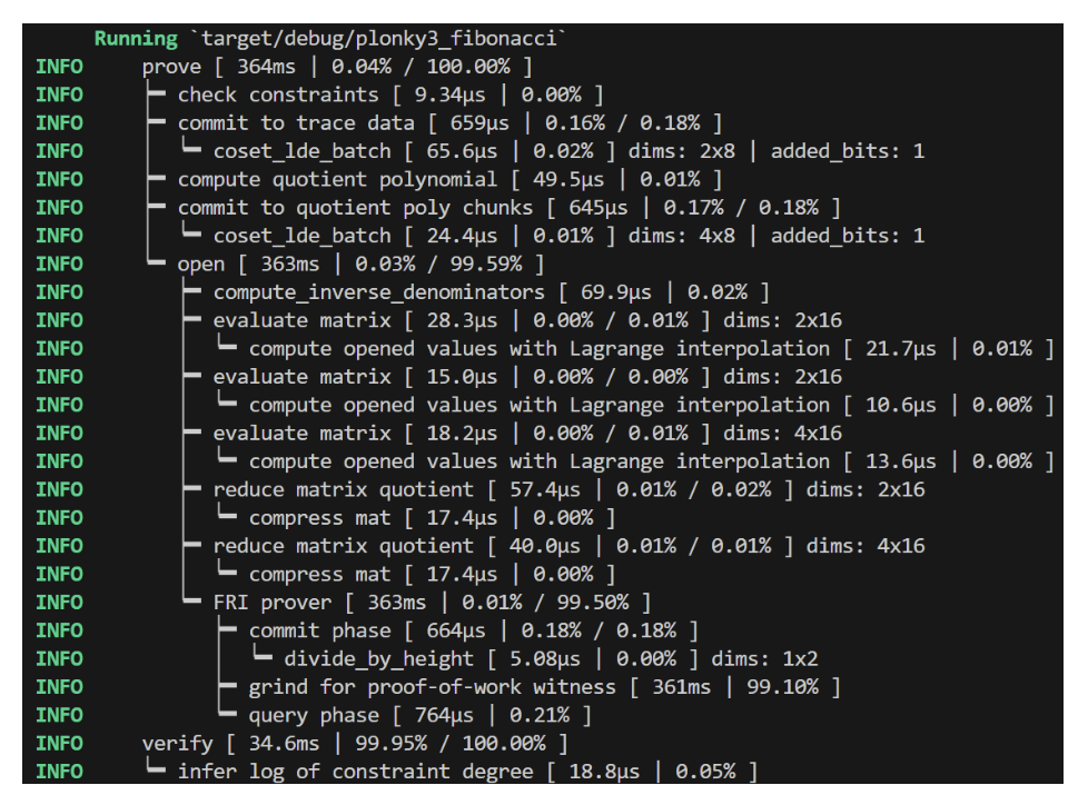
You may also notice slight differences between the logs here and those in the official documentation. This is because our example utilizes the latest Plonky3 release, along with various configuration options.
In this post, we’ll walk step by step through the Fibonacci example. By examining both the concrete prover logs and the corresponding code, we aim to demystify the Plonky3 proving process. Each step will be accompanied by references to the relevant code and the underlying theoretical concepts, giving you both a practical and conceptual understanding of how Plonky3 constructs proofs.
Commit to Trace Data
Once the execution trace of a program is generated, the prover commits to the trace polynomial. In Plonky3, the execution trace is represented as a 2D matrix (or “table”). To define this matrix, we specify two parameters:
- Width: the number of columns
- Height: the number of rows
In our Fibonacci example, we set the width = 2 and the height = 8. Importantly, the height must be a power of two (padded with zeros if not) to support the folding operations used later in the proof.
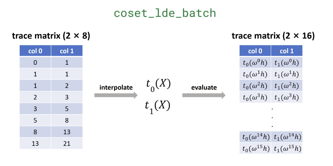
Plonky3’s prover evaluates the trace over a coset extension of the original domain, which means treating each column of the matrix as the evaluations of a polynomial on the subgroup
Why is this extension necessary? Consider it a crucial security measure. It’s easy to fake a straight line if you only have to connect two dots, but it's nearly impossible to keep up the pretense if you must plot ten more points and have them all fall perfectly on that same line. By extending the domain, we force the prover to show their work on a larger canvas, making any inconsistency or attempt to cheat far more obvious to the verifier.
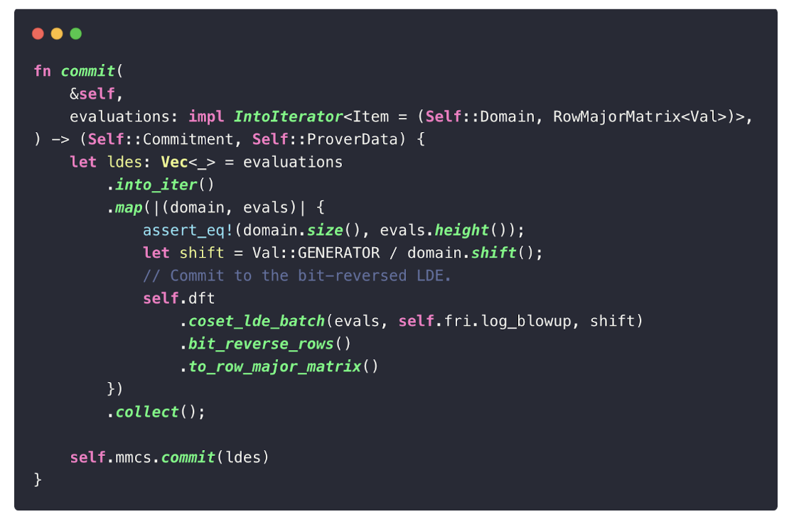
This process is implemented in the coset_lde_batch function (also used in quotient computation). The size of the coset is determined by the FRI blow-up factor, which we hard-coded in the configuration.
The core logic for committing to the trace matrix can be found in uni-stark/src/prover.rs, where pcsis the Polynomial Commitment Scheme we set:
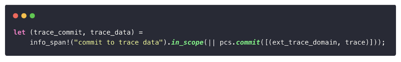
Two important functions are involved in the Polynomial Commitment Scheme phase:
coset_lde_batch: interpolates the trace matrix and evaluates the resulting polynomials over the coset.mmcs.commit: commits to the matrix using a Merkle-tree-based scheme.
For example, if we set this factor to be 1, then the new evaluation of trace will be:
Plonky3 relies on the Mixed Matrix Commitment Scheme (MMCS), a generalization of vector commitments. MMCS supports committing to entire matrices and later opening specific rows. Each row of the trace matrix is treated as a leaf node in a field-based Merkle tree. Notably, MMCS can handle matrices with varying heights, making it highly flexible.
 Source: Field Merkle Tree
For readers interested in a deeper dive, we recommend Kaneki’s blog post and this notebook for excellent explanations of MMCS in action.
Compute and Commit Quotient Polynomial
In the arithmetization system, constraints generally fall into two categories:
- Boundary constraints: enforce conditions on inputs, outputs, or other boundary values.
- Transition constraints: enforce the rules that govern state changes across computation steps.
A useful mental model is to think of each column in the trace as a register, and each row as a snapshot of the registers at a given step. Transition constraints then describe how the registers evolve from one row to the next; this is essentially how a zkVM enforces program execution.
Formally, let
Here:
- KaTeX can only parse string typed expressionencodes the transition logic.
- KaTeX can only parse string typed expressionis the vanishing polynomial, which evaluates to zero at every point in the evaluation domainKaTeX can only parse string typed expression.
After combining all constraint polynomials (including transition contstraints polynomials and boundary constraints polynomials) with random challenges, we obtain the quotient polynomial:
Where
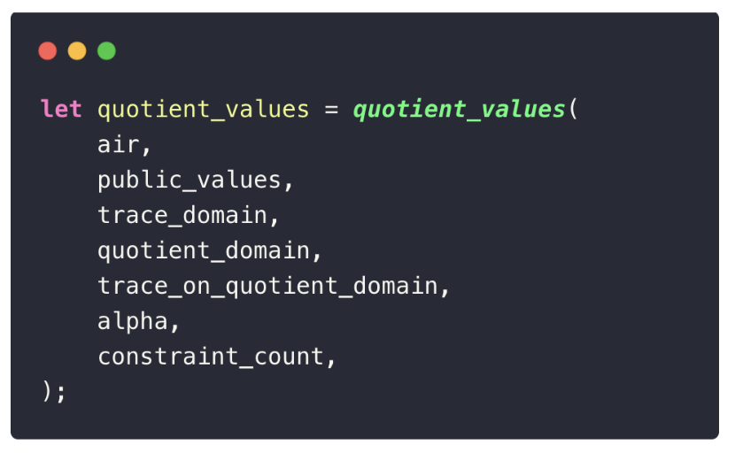
Why is the Quotient Polynomial a KaTeX can only parse string typed expression Matrix?
At first glance, it may seem that we should only end up with one quotient polynomial, and thus a
In our Fibonacci example, Plonky3 uses a degree-4 extension field of babybear, meaning each extension field element is represented as four base field elements. This “flattening” process explains why the quotient polynomial appears as a
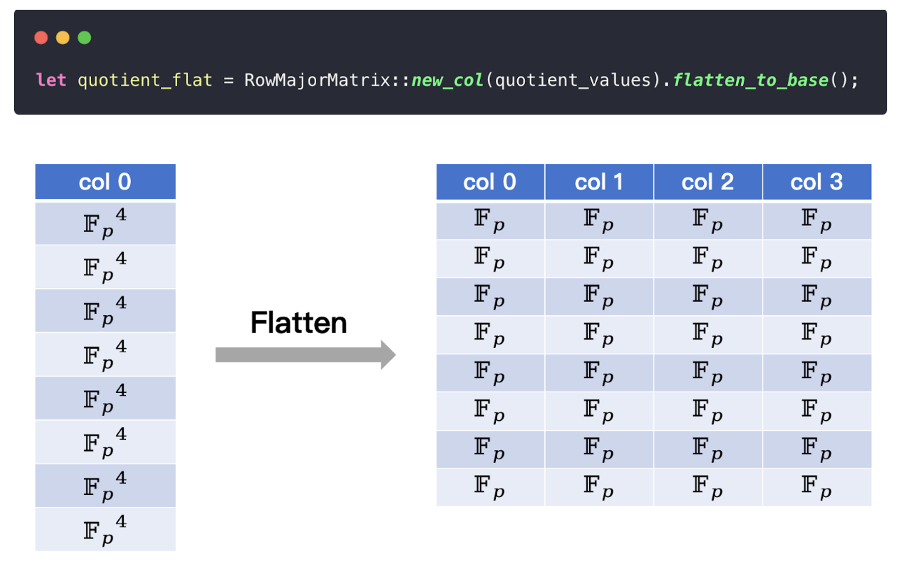
You can see this explicitly in the Fibonacci code example:
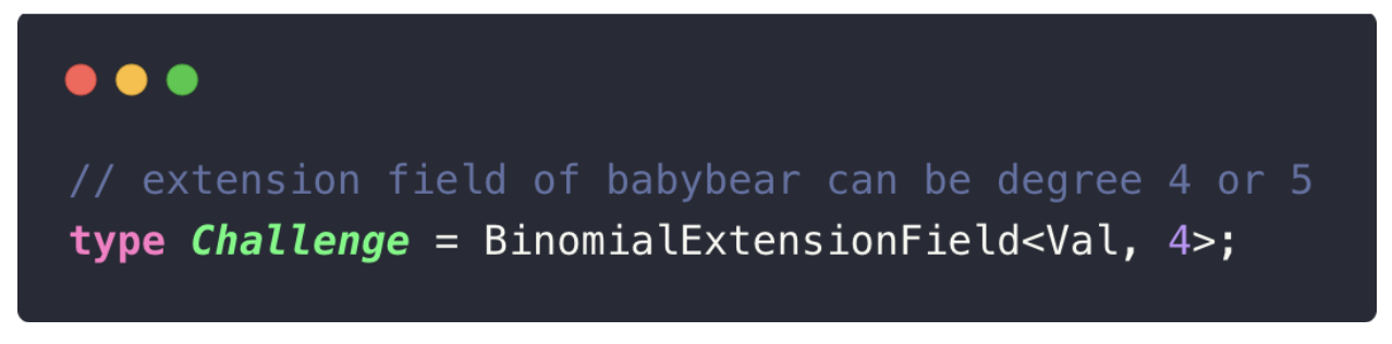
If you change this value from 4 to 5, the quotient polynomial’s dimensions expand to
Open Polynomials
The final step in the Plonky3 proving process is polynomial opening. At a high level, a Polynomial Commitment Scheme (PCS) allows the prover (committer) to reveal the evaluation of a committed polynomial
When constructing a PCS based on FRI, this check is reduced to working with the evaluation quotient:
where
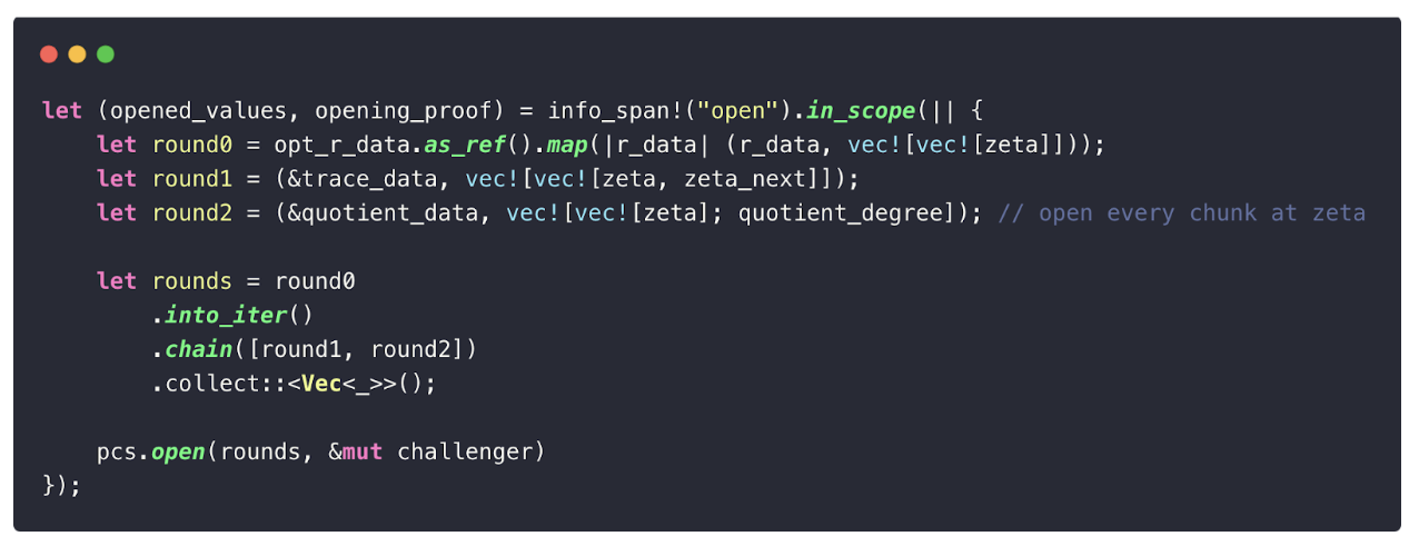
In Plonky3, the prover must open both the trace polynomial and the quotient polynomial (ignoring the random polynomial here for simplicity). The opening process can be broken down into several phases:
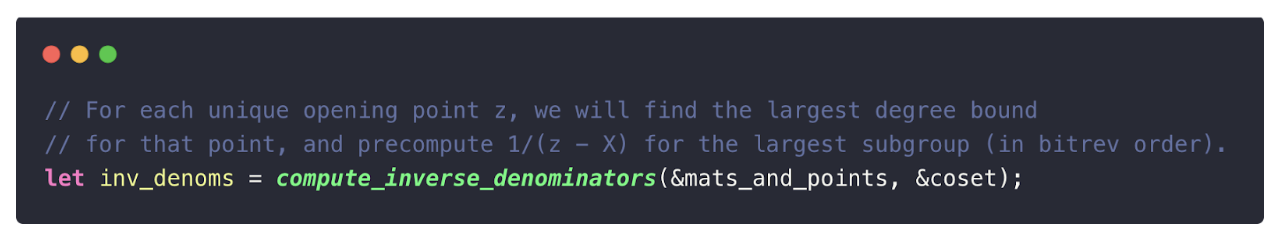
1. Compute Denominators
The denominators used in PCS openings are similar to vanishing polynomials but precomputed for efficiency. For each unique opening point
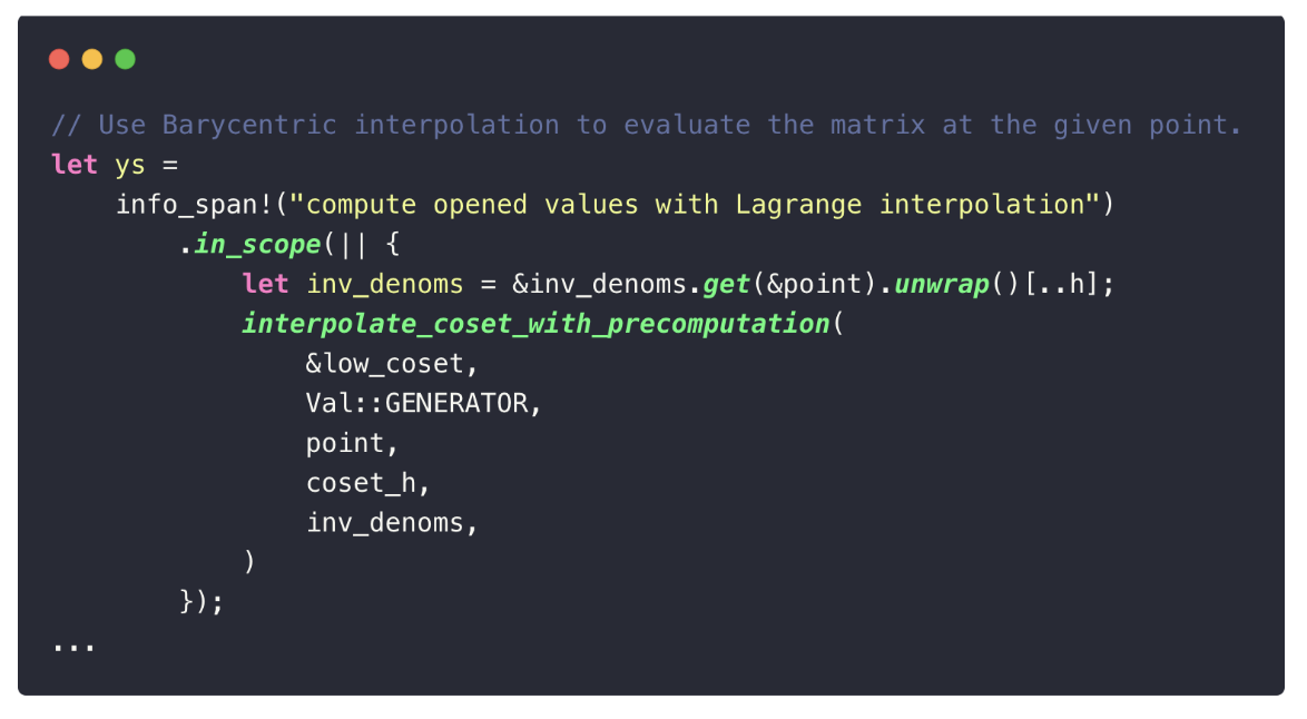
2. Evaluate Polynomials (Out of Domain)
The prover then evaluates the committed polynomials at the required points:
- Trace matrix must be evaluated at two points: KaTeX can only parse string typed expressionandKaTeX can only parse string typed expression(the shifted point). This is necessary for reconstructing the quotient polynomials, e.g.:
- Quotient matrix is evaluated at one point: KaTeX can only parse string typed expression.
In practice, this results in three calls to the evaluate_matrix function (two for the trace matrix, one for the quotient matrix), which you can observe in the prover’s logs.
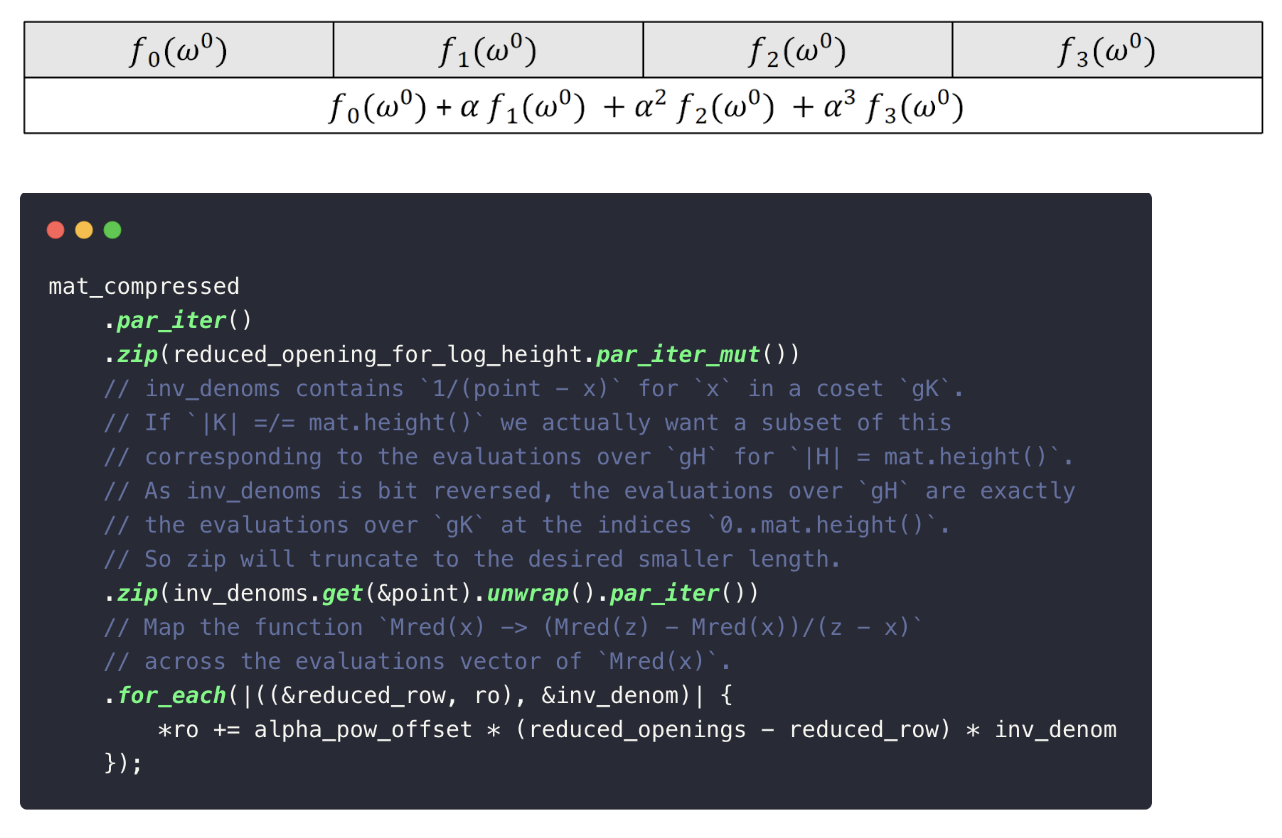
3. Compute Reduced Openings
Next, the prover constructs reduced polynomials for the FRI test:
In the Fibonacci example, there are two matrices:
- the trace matrix, giving rise to KaTeX can only parse string typed expression,
- the quotient matrix, giving rise to KaTeX can only parse string typed expression.
Since each matrix may contain multiple polynomials (depending on the width), Plonky3 uses Batch-FRI: a technique that combines all polynomial evaluations into a single instance using random challenges. This significantly improves efficiency.
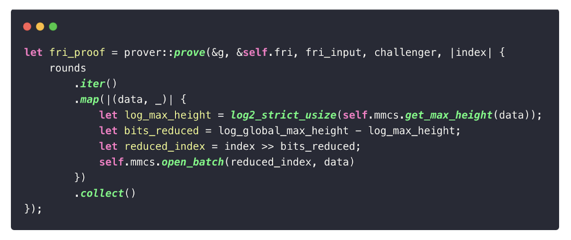
4. Generate FRI Proof
Finally, the prover runs the FRI protocol to prove that the opened polynomials are indeed of low degree. FRI works by iteratively folding the codeword (the polynomial evaluations) via random linear combinations chosen by the verifier. Each round reduces the codeword size while preserving the degree bound, until it becomes small enough to check directly.
For readers interested in the details of FRI, we recommend this documentation.
Final Proof and Conclusion
As we’ve seen, a Plonky3 proof consists of three essential components:
- Polynomial commitments – for both the trace and quotient polynomials.
- Opened evaluations – the values of these polynomials at specific points.
- Opening proofs – FRI proofs that certify the correctness of the evaluations.
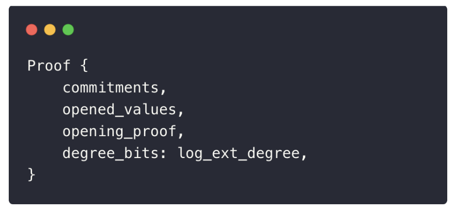
Together with the declared degree of the original trace polynomial, these elements allow the verifier to efficiently check the proof against the configuration parameters and AIR constraints.
In this post, we walked through the proving process in Plonky3 using the Fibonacci circuit as a concrete example. We explored trace commitments, quotient polynomial computation, polynomial openings, and finally, the assembly of the proof itself.
By unpacking each stage through a familiar and accessible example, our goal was to shed light on the mechanics behind zkVM proofs. While Plonky3 is often treated as a “black box,” understanding its workflow opens the door to deeper insights, optimizations, and innovations in the design of scalable zero-knowledge systems.
References and Further Reading
- STARK Prover, Lambdaclass. https://lambdaclass.github.io/lambdaworks/starks/starks.html
- ethSTARK Documentation, Eli Ben-Sasson, Dan Brownstein, Dan Carmon, Lior Goldberg, David Levit, Dori Medini, Alon Shtaierman and Eylon Yogev. https://eprint.iacr.org/2021/582
- Field Merkle Tree, Kaneki. https://hackmd.io/@0xKanekiKen/H1ww-qWKa
- eSTARK: Extending STARKs with Arguments, Héctor Masip-Ardevol, Marc Guzmán-Albiol, Jordi Baylina-Melé and Jose Luis Muñoz-Tapia. https://eprint.iacr.org/2023/474
- DEEP-FRI: Sampling Outside the Box Improves Soundness, Eli Ben-Sasson, Lior Goldberg, Swastik Kopparty, and Shubhangi Saraf. https://eprint.iacr.org/2019/336
- A summary on the FRI low degree test, Ulrich Haböck. https://eprint.iacr.org/2022/1216